Contingency table

Contingency table and chi squared distributions are used to determing if two categorical varibles are independent or not.

For example: The following table shows a contingency table of driver behaviour at stop signals based on gender.

	Male	Female
Stop	20	15
Slow down	11	12
Don’t slow down	7	9

Now the goal is to determine whether the behaviour at stop signal is gender dependent or not.

The steps to solve this problem are

Come up with a null hypthesis and expected values for all the columns.
Find the normalized squared deviations for each column.
Sum the deviation to find the chi-squared distance.
From the chi-squared distribution, find out the statistical significance of this deviation.

1. Null hypothesis

In inferential statistics, the null hypothesis is a general statement or default position that there is no relationship between two measured phenomena, or no association among groups.

In our example, the null hypothesis is : gender and behaviour are independent of each other.

2. Normalized squared deviation

import pandas as pd

df = pd.DataFrame([[20,15],[11,12],[7,9]], index=['stop','slow','noslow'], columns=['male','female'])
original_df = df.copy()

df['total'] = df.sum(axis = 1)
df.loc['total'] = df.sum(axis=0)
df

	male	female	total
stop	20	15	35
slow	11	12	23
noslow	7	9	16
total	38	36	74

For the null hypothesis to be true, the fraction of males and females should be same across all the behaviours. That’s how we will calculate our expected values for the null hypothesis.

How to calculate the expected value?

for each cell, we multiply the row sum by the column sum and divide the result by the total number of observations

df.loc['fraction'] = df.loc['total']/df['total'].loc['total']

def highlightrow(series, rowsToHighlight):
    return ['background-color: yellow']* len(series) if series.name in rowsToHighlight else ['']* len(series)
df.style.apply(highlightrow,axis = 1, rowsToHighlight='fraction')

	male	female	total
stop	20	15	35
slow	11	12	23
noslow	7	9	16
total	38	36	74
fraction	0.513514	0.486486	1

df['male'] = df['total'] * df['male'].loc['fraction']
df['female'] = df['total'] * df['female'].loc['fraction']
df = df.drop(labels=['total','fraction']).drop(columns = ['total'])
expected_df = df
expected_df

	male	female
stop	17.972973	17.027027
slow	11.810811	11.189189
noslow	8.216216	7.783784

3. Chi-squared distance

The chi-squared distance calculates how much the observed frequency deviates from the expected frequency. Chi squared distance is the sum of normalized square deviation of all the observations.

$\sum_{1}^{n} {\frac{(O-E)^2}{E}}$

deviations = (original_df - expected_df )**2/df
deviations

	male	female
stop	0.228612	0.241313
slow	0.055662	0.058754
noslow	0.180032	0.190034

chi_distance = deviations.sum().sum()
chi_distance

0.9544070774762996

4. Statistical significance

A set of categorical variables will always have some variation in the behaviour. For example if we toss a coin 100 times, the expection is to get 50 heads and 50 tails. Butwe might get 51 heads and 49 tails. Still we dont think, there is something odd with the coin as the deviation is not statistical significance.

Similarly, for our example, we find the chi-squared deviation to be 4.97. But how do we know if this deviation is significant or not!!

For that we will use two concepts.

Chi-squared distribution
Degrees of freedom

chi-squared distribution is the probability distribution of chi squared distances for k degrees of freedom.

If our null hypothesis was true, then the chi squared distance, if we repeat the experiment multiple times, will be distributed according to the chi-squared distribution.

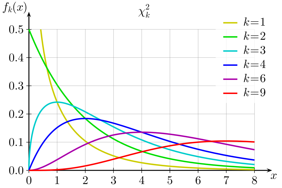
Our example has only 2 degree of freedoms as all the other values can be derived from the row and column totals. Now let’s calculate, what’s the probability of getting chi squared distance of 0.9544 if our null hypothesis was true(i.e. gender and behaviour are independent).

The green line (k=2) from the above graph constitutes the distribution for 2 degrees of freedom. As evident, the probability of getting a chi squared distance >= 0.9544 will be the area under the green line for x>0.9544.

To calculate the exact number, a library called scipy can be used.

from scipy.stats import chi2
1 - chi2.cdf(chi_distance, 2)

0.6205162173513055

Hence there is 62% possibility of getting a deviation bigger than 0.9544. That means our null hypothesis is correct.

Shortcut

The entire calculation could also have been done using a single command.

from scipy.stats import chi2_contingency
chi2_contingency(original_df.values)
#help(chi2_contingency)

(0.9544070774762996, 0.6205162173513055, 2, array([[17.97297297, 17.02702703],
        [11.81081081, 11.18918919],
        [ 8.21621622,  7.78378378]]))

Conclusion

The contingency table analysis using chi-squared distance proves that human behaviour at stop signs is independent of gender.