Insertion transformer summary

Insertion Transformer paper

An iterative, partially autoregressive model for sequence generation based on insertion operations.

Abstract

Advantages:

1. It can be trained to maximize entropy over all valid insertions for robustness.

2. It can do multiple insertions at a time

Outperforms non-autoregressive approaches. On par with transformer based AR models with exponentially small number of iterations.

Content location distribution

To calculate the joint probability over both the next location and content, this paper has proposed 2 approaches.

1. Joint distribution

    p(c, l) = softmax(flatten(HW))
    p(c, l) = probability of content c at location l
    H -> R (T +1)×h 
    h is the size of the hidden state
    T is the length of the current partial hypothesis
    W -> R h×|C|  the standard softmax projection matrix
    C is vocabulary size
   
    This takes the combination of all available  slots and content and calculates joint probablity.
   

2. conditional factorization

    p(c, l) = p(c | l)p(l)
    p(c | l) = softmax(hlW)
    This softmax is applied per slot. 
    p(l) = softmax(Hq)
    q is a trainable vector.
    This softmax gives the probability of slot l.
   

In both the cases, the probability os over all the available slots. During training, only

Previous approaches

1. Neural sequence model
   • autoregressive left-to-right structure.
   • No paralleliation during inferncing

2. Non-Autoregressive Transformer (NAT) (Gu et al., 2018) and the Iterative Refinement model (Lee et al., 2018)

   Sequences are predicted all at once followed by optional refinement stage. Highly parallel but comes with few drawbacks.

    1. Target sequence length needs to be determined upfront prevents further growth of target sequence.
    2. Output tokens are assumed independent which is not right. The refinement stage handles this problem partially.
   

Training and Loss Functions

1. Left to right

   Only one output is produced at a time . It imitates traditional left to right auto regressive models.

   To do so, given a training example (x, y), we randomly sample a length k ∼ Uniform([0, |y|]) and take the current hypothesis to be the left prefix yˆ = (y1, . . . , yk). We then aim to maximize the probability of the next content in the sequence c = yk in the rightmost slot location l = k, using the negative log-likelihood of this action as our loss to be minimized:

   loss(x, yˆ) = − log p(yk+1, k

   x, yˆ)

2. Balanced Binary Tree

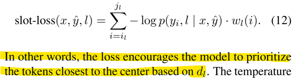
   Weight is added to losses for targets in the middle of the slots.

   

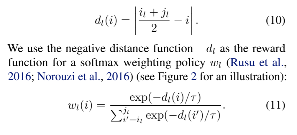
   • i = Current span position.
   • i_l =starting position for current span for location l
   • j_l =starting position for current span for location l

   As d_l will be minimum if i = middle of the span. Hence w_l(i) will be high for span positions(i) which are in the middle of the sequence.

   Example

   Original [A,B,C] D [E,F,G]
   Predicted canvas is only D till now

   For l = 0, Span = A,B,C

   For l =1 , span = E, F, G
   i1 = 4
   j1 = 6

   For soft binary, we want the insertion transfer to give weightage to slot 5 for l = 1

   Hence the softmax will assign high weight to slot 5 in this case.

   

   Now if next iteration does not predict 5 the loss will be very high

3. Uniform

   Same as balanced tree. But the weight w is 1 for every location in a span. Giving the model unbiased chance to predict next location. But this will increase overall loss as only only location is predicted for a span in one iteration. Hence the loss might not converge to zero but should still converge to a minimum value.

Termination

2 approaches for termination

1. Slot finalization
2. Sequence finalization